Detecting Graph Symmetries

The goal of this project was to develop a computer program for detecting symmetries in vertex-colored undirected graphs. The program should mimic the algorithms in the saucy symmetry detection system. The saucy page was consulted for papers that describe how saucy works and give worked-out examples tracing the execution of the saucy algorithm. In what follows we will call the program saucy_clone.

0. TLDR;

0. a. A quick presentation

0. b. Project Link

Presentation Link

1. Introduction and Background

One source of intractability in SAT is the presence of structural symmetries in the solution space. In this context, a symmetry is a permutation of the literals of a CNF formula that leaves the formula unchanged. The symmetries of an $n$-variable formula induce an equivalence partition on the formula's $2^n$ possible truth assignments. The assignments in a given cell of such a partition are equivalent in the sense that the formula evaluates to the same truth value (either 0 or 1) on all of them. So rather than search in the space of the $2^n$ possible assignments, a SAT solver could be directed to search in the much smaller space of the equivalence partition. This approach is generally referred to as $symmetry\enspace breaking$ and it has many variants. In particular, $static$ symmetry breaking consists of the following steps:

Convert the CNF formula to a colored graph
Find (some of) the symmetries of the graph (defined below)
For each such symmetry, create a $symmetry-breaking\enspace predicate$ (SBP) in CNF
Conjoin the SBPs to the original formula and pass the augmented formula to the SAT solver

This approach to symmetry breaking has led to dramatic pruning of the search space in some cases. In particular, it works extremely well for pigeon hole instances (unsatisfiable CNF formulas that encode placing $n + 1$ pigeons in $n$ holes such that no hole has more than one pigeon). But in many cases the reduction in the size of the search space does not translate to a reduction in run time due to the overhead introduced by the SBPs.

In any case, this project is not about symmetry breaking for SAT. Rather, as often happens in research, the unexpected foray into symmetry detection in graphs led to the development of the saucy program which differs in fundamental ways from earlier symmetry detectors and achieves an unprecedented six orders of magnitude performance edge.

Before embarking on this project it is highly advisable that you read the following references:

K. A. Sakallah, “Symmetry and Satisfiability,” in Handbook of Satisfiability. vol. 185, A. Biere, et al., Eds., ed: IOS Press, 2009, pp. 289-338. PDF
H. Katebi, K. A. Sakallah, and I. L. Markov, “Symmetry and Satisfiability: An Update,” in Thirteenth International Conference on Theory and Applications of Satisfiability Testing (SAT), Edinburgh, 2010, pp. 113- 127. PDF PPT

In addition, you should consult the saucy webpage for additional references and links to related work.

The project is designed to have a sequence of well-defined deliverables that insure progress towards the final “product” which is a saucy clone.

2. Graph Input Format

The vertices of an $n$-vertex $c$-color undirected graph are assumed to be numbered consecutively from $0$ to $n−1$. The $c$ colors partition the vertex set into $c$ different cells such that vertices in any given cell share the same color. In addition, it is assumed that vertices of the same color are numbered consecutively with no gaps (see example below). A graph input file is a text file consisting of a header followed by a listing of the graph edges. All fields in the input file should be decimal integers. White spaces, including newlines, serve as field separators and are ignored. The file header for a graph that has $n$ vertices, $e$ edges, and $c$ colors has the following format:

$$ n\quad e\quad c \quad v_2\quad v_3\quad ...\quad v_{c−1} $$

$$ \text{Figure 1: Example Graph and its Input Format} $$

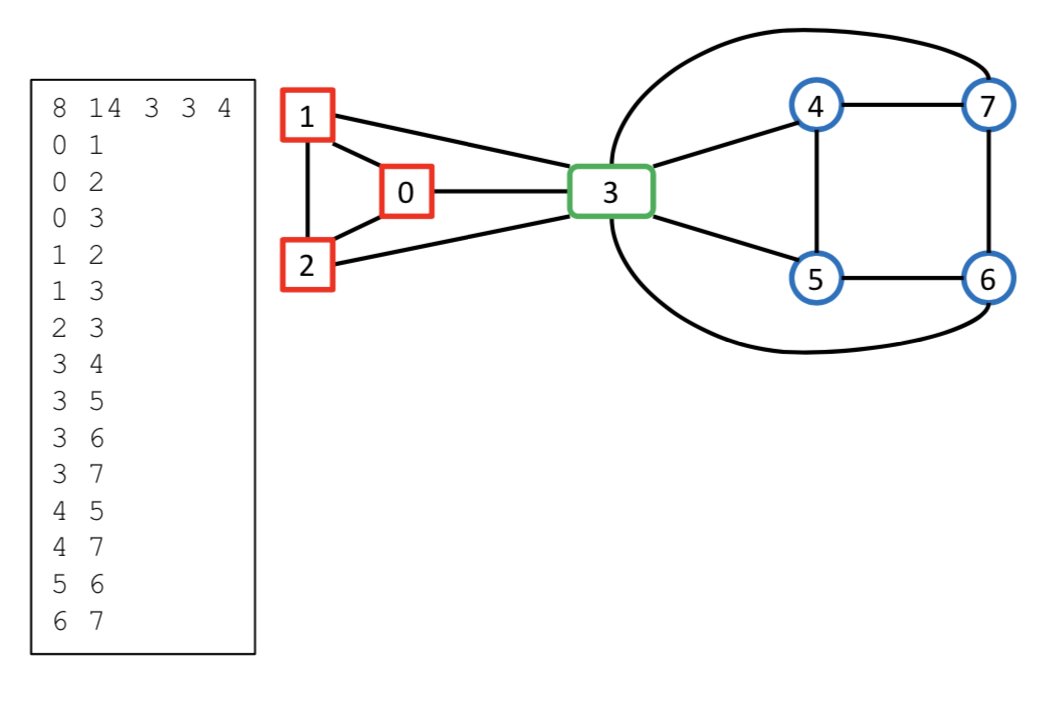
where $v_i$ is the index of the least vertex in the cell corresponding to color $i$. In what follows we will refer to $n\enspace e\enspace c \enspace v_2\enspace v_3\enspace ...\enspace v_{c−1}$ as the color change locations. For example, the header

$$ 8\enspace 14\enspace 3\enspace 3\enspace 4 $$

describes a graph with $8$ vertices, $14$ edges, and $3$ colors. The colors partition the set of vertices into the following three disjoint subsets: $[\enspace 0\enspace 1\enspace 2\enspace \vert\enspace 3\enspace \vert\enspace 4\enspace 5\enspace 6\enspace 7\enspace ]$. The last two numbers in the header indicate that color $2$ starts at vertex $3$ whereas color $3$ starts at vertex $4$; they also implicitly indicate that color $1$ applies to all vertices numbered lower than $3$. Note that when $c = 1$ the list of color change locations is empty. Graph edges are specified as pairs of vertices given in either order (since the graph is undirected). Note also that the order of edges in the listing is unimportant. An example colored graph and its associated input file are shown in Figure 1.

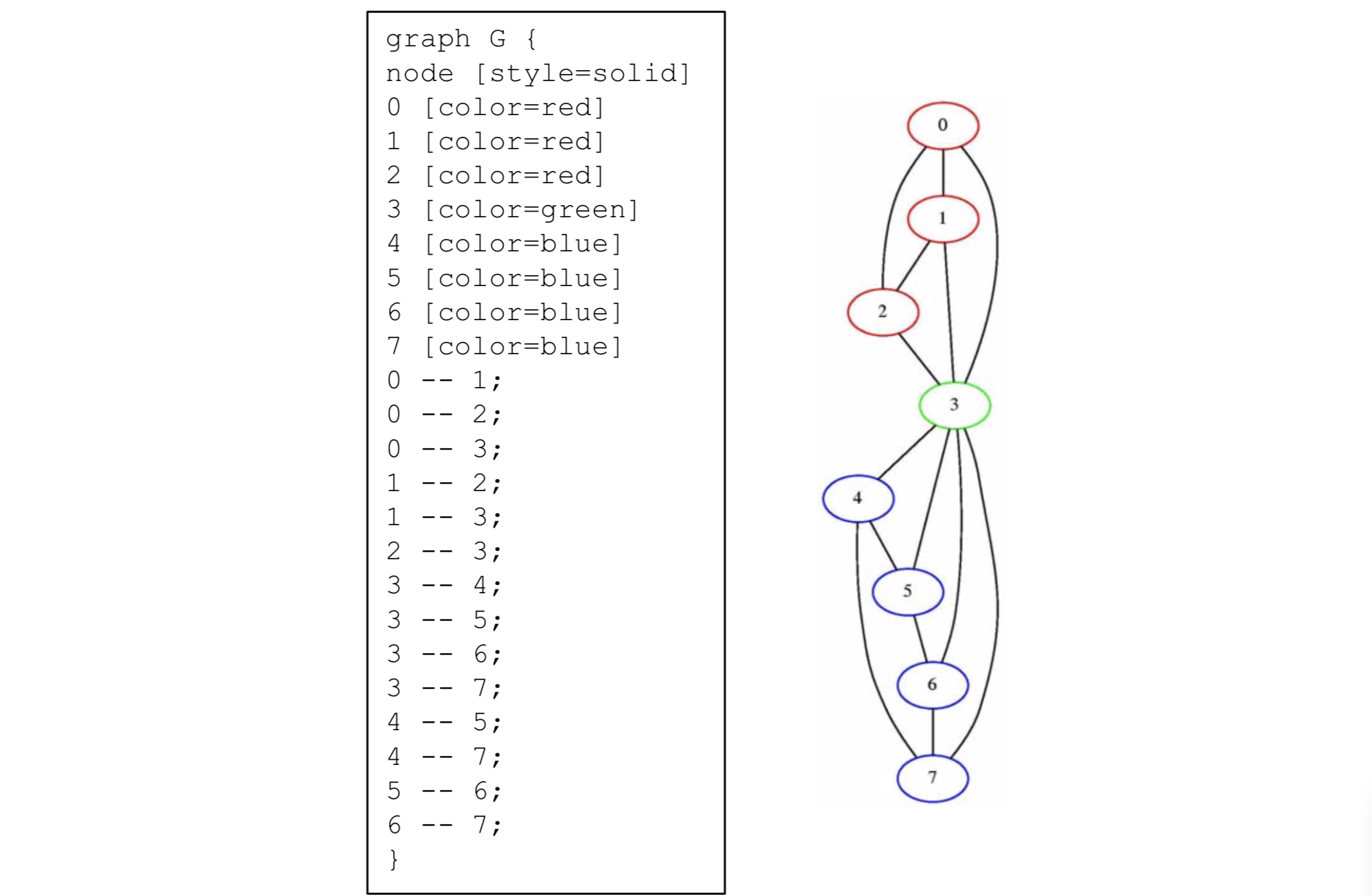
A useful tool for drawing graphs is Graphviz which can be downloaded from here. The input text format and graphical output format of Graphviz for the graph of Figure 1 are shown in Figure 2.

3. Representation of Vertex Permutations

Permutations are typically expressed in one of two ways: tabular form or $cycle\enspace notation$. For example, given the set ${0,1,2}$ the permutation that maps $0$ to $1$, $1$ to $2$, and $2$ to $0$ can be expressed as the table

$$ \left[ \begin{array}{c|c|c} 0 & 1 & 2 \ 1 & 2 & 0 \ \end{array} \right] $$

$$ \text{Figure 2: Graphviz input and output for the graph of Figure} $$

or as the cycle $(0\enspace 1\enspace 2)$. Cycle notation is very compact when the number of vertices moved by a permutation is much smaller than $n$. The output of saucy is a set of (at most $n−1$) $generators$ expressed in cycle notation. Generators are vertex permutations that, when combined in all possible ways, are guaranteed to yield all possible graph symmetries. Within saucy, the basic data structure for encoding permutations is the so-called $Ordered\enspace Partition\enspace Pair$ (OPP) which is a generalization of tabular notation that allows for the implicit encoding of a set of permutations. This is detailed in here. The OPP data structure is key to the way that saucy searches for symmetries in the permutation space whose size, for a graph with $n$ vertices, is $n!$.

Here are several example OPPs and the permutation sets they encode.

Discrete OPP: $$ \left[ \begin{array}{c|c|c} 2 & 0 & 1 \\ 1 & 2 & 0 \\ \end{array} \right] = \{ (0\enspace 2\enspace 1 ) \} $$
Unit OPP:

$$ \begin{bmatrix} 0,1,2 \\ \\ 0,1,2 \end{bmatrix} = \{ι,(0\enspace 1),(0\enspace 2),(1\enspace 2),(0\enspace 1\enspace 2),(0\enspace 2\enspace 1)\} $$

Isomorphic OPP:

$$ \left[ \begin{array}{c|cc} 2 & 0,1 \\ 1 & 2,0 \end{array} \right] = \{(1\enspace 2),(0\enspace 2\enspace 1)\} $$

Matching OPP:

$$ \left[ \begin{array}{c|c|c} 1 & 0,2,4 & 3 \\ 3 & 0,2,4 & 1 \end{array} \right] = (1\enspace 3) \circ S_3 ({0,2,4}) $$

Non-isomorphic OPPs:

$$ \left[ \begin{array}{c} 0,2\vert 1 \\ \\ 1\vert 2,0 \end{array} \right] = \emptyset , \left[ \begin{array}{c} 2\vert 0\vert 1 \\ \\ 1\vert 2,0 \\ \end{array} \right] = \emptyset $$

4. Data Structure for Ordered Partitions

A lot of what saucy does involves the manipulation of ordered partitions (OPs), primarily refining (i.e. splitting) cells by changing the positions of the affected vertices. To do this efficiently, saucy uses a $Vertex\enspace Array$ to store the vertices of the OP along with three other “helper” arrays to keep track of cell boundaries and lengths:

To enhance readability, the names used here are not the same as in the saucy source code

Vertex[$i$] is the number of the vertex located at position $i$ in the OP
Position[$v$] is the position in the Vertex array at which vertex $v$ is located
CellFront[$v$] is the position in the Vertex array corresponding to the first vertex in the cell containing vertex $v$
CellSize[$f$] is one less than the size of the cell that begins at position $f$ in the Vertex array

As an example, the OP $$ \left[ \begin{array}{c|c|c|c} 3 & 2,4 & 1,5 & 0,6 \end{array} \right] $$

is encoded as:

$$ \begin{array}{c|c,c,c,c,c,c} Position,i & 0 & 1 & 2 & 3 & 4 & 5 & 6 \\ \hline Vertex[i] & 3 & 2 & 4 & 1 & 5 & 0 & 6 \end{array} $$

$$ \begin{array}{c|c,c,c,c,c,c} Vertex,v & 0 & 1 & 2 & 3 & 4 & 5 & 6 \\ \hline Position[v] & 5 & 3 & 1 & 0 & 2 & 4 & 6 \end{array} $$

$$ \begin{array}{c|c,c,c,c,c,c} Vertex,v & 0 & 1 & 2 & 3 & 4 & 5 & 6 \\ \hline CellFront[v] & 5 & 3 & 1 & 0 & 1 & 3 & 5 \end{array} $$

$$ \begin{array}{c|c,c,c,c,c,c} CellFront,f & 0 & 1 & 2 & 3 & 4 & 5 & 6 \\ \hline CellSize[f] & 0 & 1 & - & 1 & - & 1 & - \end{array} $$

Strictly speaking the Position array is not needed as it is just the “inverse” of the Vertex array, but it does speed up OP processing. The slightly mis-named CellLength array is defined as described above so that singleton cells can be identified quickly by checking if their corresponding entry in CellLength is 0. In addition, CellLength is defined only at the positions corresponding to cell fronts.

As an example of using this data structure, given a vertex $v$, its position in the OP is $Position[v]$, its cell starts at position $CellFront[v]$, and the size of the cell is $1 + CellSize[CellFront[v]]$.

5. Deliverable I–Parser for Input Format

The goal of this deliverable is to write a parser for the text format for encoding colored graphs described in Section 2. This parser should do the following:

Read an input graph
Store the graph in a linked-list data structure
Write out the graph in the same format to insure that it matches the input
Write out the graph in the Graphviz format and run it through Graphviz to draw it

For extra bonus, the output may also contain statistics about the graph such as the color degree of each vertex (how many neighbors a vertex has of a certain color).

6. Deliverable II–Partition Refinement

The goal of this deliverable is to implement the vertex partition refinement procedure which is the main mechanism for distinguishing non-symmetric vertices in the graph. Consider an ordered partition $\pi = \left[ W_1\vert W_2\vert \dots \vert W_k \right]$ of the graph vertices and let $d(v,W_i)$ be the $color-relative\enspace vertex\enspace degree$ of vertex $v$ with respect to cell $W_i$ of the partition. Specifically, $d(v,W_i)$ is the number of vertices in cell Wi that are adjacent to v (i.e., the number of connections v has to cell Wi). An ordered partition is $equitable$ if all vertices in each cell of the partition have the same color-relative vertex degree. Partition refinement is triggered if the partition is not equitable, meaning that a vertex in some cell of the partition has a color-relative degree that is different from the color-relative degrees of the rest of the vertices in that cell. That vertex can, thus, be distinguished by separating it from the other vertices in the cell to obtain a $finer$ partition (i.e., one that is obtained by splitting some of its parent partition cells). The resulting partition may still be inequitable, triggering another round of splitting. This process continues until an equitable partition is obtained. The core operation in partition refinement is the (potential) splitting of a $target$ cell $T$ by an inducing cell $I$. This is done by computing the degrees of $T$'s vertices relative to $I$ and creating a partition of $T$ such that each of its cells has vertices with the same degree relative to $I$. This operation, which we will call refine_cell, takes the current partition $\pi$ along with the target and inducing cells, and returns a (potentially) $finer$ partition $\hat\pi$ and a (potentially empty) list of “new” cells that form a partition of $T$ : The refinement procedure can now be implemented by maintaining a queue $Q$ of inducing cells which are processed one at a time by refine_cell. If this causes a target cell to be split, its parts are inserted in the queue for later processing. Given an initial queue of inducing cells, the pseudo code for partition refinement is roughly as follows:

refine (OP P) {
  while not empty(Q) {
    I = pop(Q);
    for each cell T with connections to I {
      (OP P, Cell List L) = refine_cell(OP P, cell T, cell I);
      if not empty(L) {
        if T is in Q, remove it;
        for each cell t in L
          push(t, Q);
      }
    }
  }
}

Note that there are many optimizations that can make this procedure more efficient. In particular, saucy maintains a separate queue of singleton inducing cells and processes that queue before it processes the queue of non-singleton cells. In addition, saucy eliminates the step of removing from the queue a target cell that also happens to be an inducing cell (line 06). This does not affect the correctness of the procedure: if refinement splits cell $T$ into, say $T1$ and $T2$, the queue will now contain two copies of $T1$ (assuming it is the left cell) since $T$ no longer exists! Having duplicate copies of refining cells in the queue causes no harm other than repeating the connectivity checks to other target cells. For very large sparse graphs such checks are much less expensive than locating and removing a cell from the queue.

An example of partition refinement is shown in Figure 3. The initial unit partition in $(a)$ is refined to the 2-cell partition in $(b)$ based on vertex degrees. The two cells of partition $(b)$ are then inserted into $Q$, the inducing cell queue. The cell at the top of the queue, ${1, 2, 3, 4, 5}$, is now popped and used to refine the target cell ${0, 6}$. Since the number of connections of vertices 0 and 6 to the inducing cell are equal, cell ${0, 6}$ cannot be refined. The next inducing cell at the top of the queue is ${0, 6}$, and when used to refine target cell ${1, 2, 3, 4, 5}$, it splits it into two cells,${1, 5}$ and ${2, 3, 4}$, yielding partition $(c)$. Continuing in this fashion, the algorithm terminates after a few more steps producing the final equitable partition $(d)$.

The implementation of partition refinement in saucy includes several optimizations that help to reduce its computational complexity. For example, singleton cells need not be “touched” during refinement since they cannot be split. In addition, saucy applies partition refinement $simultaneously$ to both the top and bottom partitions of an OPP.

For this deliverable, we wrote a partition refiner that does the following:

Read a colored graph (using the parser developed in deliverable I)
Create an initial Ordered Partition Pair (OPP) using vertex degrees to place vertices into different cells
Refine the OPP (top and bottom) until it becomes equitable
Write out the initial OPP and the OPP after each refinement iteration

7. Deliverable III–Subgroup Decomposition

The goal of this deliverable is to construct the left-most branch of the permutation search tree. This branch is referred to as subgroup decomposition. Starting at the root of the tree and at subsequent levels, $$subgroup\enspace decomposition$$ involves the following steps:

Selecting a non-singleton $$target\enspace cell$$ from the current OPP
Selecting a $$target\enspace vertex$$ from the target cell
Forcing that vertex to map to itself by splitting it from its current cell in both the top and bottom partition of the OPP
Refining the resulting OPP

The queue actually contains the cell fronts of cells, and so will have a duplicate cell front.

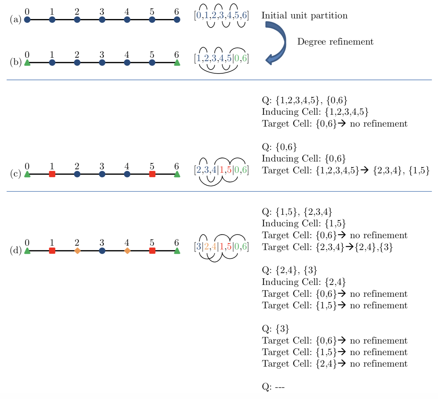
$$ \text{Figure 3: Example of Partition Refinement} $$

An example of subgroup decomposition is shown in Figure 4. The OPP at the root of the search tree corresponds to (an uncolored version of) the graph of Figure 1. It consists of two cells obtained by separating the graph vertices based on their degree. The first $decision$ in this decomposition is to map vertex $4$ to itself which yields an OPP that is not equitable. This triggers two refinement iterations that result in splitting the only non-singleton cell in the OPP into three cells, separating vertices $5$ and $7$, and then $6$ from the other vertices. The second decision maps vertex 5 to itself but does not trigger further refinement. Similarly, the last two decisions map 0 to itself and 1 to itself yielding the final discrete OPP that corresponds to the identity permutation.

For this deliverable, we wrote a subgroup decomposition program that does the following:

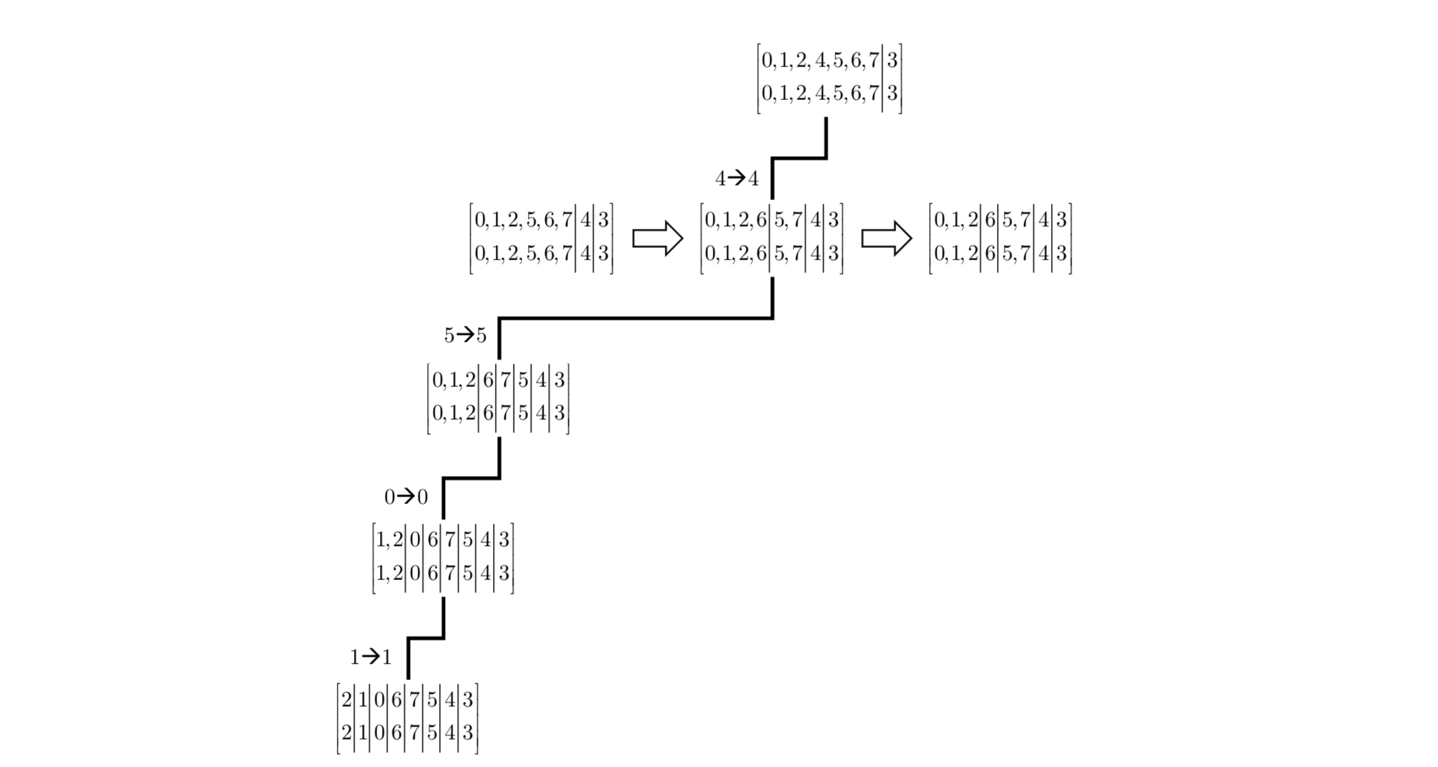
$$ \text{Figure 4: Example of Subgroup Decomposition for Graph in Figure} $$

Read a colored graph (using the parser developed in deliverable I)
Create and refine an initial Ordered Partition Pair (OPP) (using the partition refiner in deliverable II)
Construct a subgroup decomposition “tree” similar to that in Figure 4 Write out, at each level of the decomposition:
- The initial OPP corresponding to the vertex selected to be mapped to itself
- The sequence of OPPs obtained through partition refinement
- The number of permutations encoded by the last equitable OPP

8. Deliverable IV–saucy clone

To complete the cloning of saucy, we had to construct and traverse a permutation search tree. The first part of the tree is the left-most subgroup decomposition path we developed in deliverable III. Each node along that path encodes a subgroup $$stabilizer$$, i.e., a subgroup that “fixes” the vertex chosen at that level. To complete the tree, the other possible mappings of that vertex must be explored and each such mapping can lead to a subtree in the search space that may or may not contain valid symmetries. Under each such mapping, the search must continue until a permutation that pre- serves the graph edge relation is found, or until it can be shown that no such permutation exists. The full details of this search algorithm can be found in here which should be reviewed carefully before embarking on the implementation.

For this deliverable we wrote a program called saucy_clone which includes the following modules:

A parser for colored graphs (deliverable I)
A partition refiner (deliverable II)
A subgroup decomposer (deliverable III)
A procedure to check if a given permutation is a graph symmetry (apply permutation to graph and check if edge relation is unchanged)
A search procedure that incorporates the following four pruning techniques which are described in detail in the above reference:
- Coset pruning
- Orbit Pruning
- Matching OPP
- Non-isomorphic OPP
A procedure to write out the symmetries found and any other useful statistics

saucy_clone was tested on a set of graphs and its results compared to those produced by saucy.

Love,
Ahmed Jazzar